Getting Started With High-Level Tensorflow
TensorFlow is one of the main tools used in the industry to perform Machine Learning (ML), either using it at a low-level for graph computation, or at a high-level to create models using pre-defined building-blocks. The latter is the most common approach when learning to build and train ML models.
Motivation
In this article I’ll explain how to use TensorFlow at a High-level in order to build a model that is capable of identifying the sentiment of a comment as either positive or negative. The article will be driven by the following questions: what?, why?, and how?
I just described the first one: what we are building is a model that can predict the sentiment of a comment. Now, why would this be useful? Well, as an example, let’s say you want to know how your brand is performing on social networks. Are customers happy about you? In order to answer that question you may hire a Community Manager to analyze hundreds/thousands of comments to give you an answer. That would be both time consuming and expensive, moreover, if you perform such tasks periodically, then you should think of a better strategy to handle this. A possible strategy could be to create a ML model that can handle that task for you, saving you a lot of time and money. Having answered the what and why, let’s use the rest of the article to explain the how.
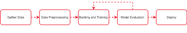
A (Very) Summarized Representation of a ML Experiment
In order to get some background on what we are going to do, I created this diagram that explains what’s the common protocol to follow when performing a Machine Learning experiment. It’s just a very (very) general idea and each step involves a lot more work, so this is an oversimplification.
Requirements
- An environment with TensorFlow installed. I’ll use Google Colab so I suggest you to do the same so you don’t have to install or set up anything.
- The code will be based on the official TensorFlow documentation, with several modifications.
Go to Google Colab and create a new notebook. Then, put this starting code in the first cell:
!pip install -q kaggle pyyaml

import matplotlib.pyplot as plt
import TensorFlow as tf
from TensorFlow import keras
from TensorFlow.keras import layers
from collections import Counter
import numpy as np
import seaborn as sns

class Utils:
  # A dictionary mapping words to an integer index
  INDEX = imdb.get_word_index()
  INDEX = {k:(v+3) for k,v in INDEX.items()} # The first indices are reserved
  INDEX["<PAD>"]    = 0
  INDEX["<START>"]  = 1
  INDEX["<UNK>"]    = 2  # unknown
  INDEX["<UNUSED>"] = 3

  PAD_VALUE = INDEX["<PAD>"]

  REVERSE_INDEX = dict([(value, key) for (key, value) in INDEX.items()])

  @classmethod
  def decode_review(cls, text):
      return ' '.join([cls.REVERSE_INDEX.get(i, '?') for i in text])

  @classmethod
  def plot(cls, history=None, series=None, title=None):
    PARAMS = dict()
    PARAMS['acc'] = dict(label="Training Acc", )
    PARAMS['val_acc'] = dict(label="Validation Acc", )
    PARAMS['loss'] = dict(label="Training Loss", )
    PARAMS['val_loss'] = dict(label="Validation Loss", )

    epochs = range(1, len(history[series[0]]) + 1)

    for serie in series:
      plt.plot(epochs, history[serie], **PARAMS[serie])
      print(f"Max {serie}: {max(history[serie])}")

    plt.title(title)
    plt.xlabel('Epochs')
    plt.legend()

    plt.show()

NUM_WORDS = 10000
Gather Data
We collect samples to train the model. We’re performing “supervised classification” so data should be “labeled”. Labeled data contains examples with a priori predictions of what we want to learn, meaning that we will have samples of comments along with their related labels (positive or negative). It could be seen as: “I have these comments, this one is positive, this other is negative, this one seems to be also negative, …”
Quite often, labeling data is performed manually and it consumes a lot of time. If we’d have to do it, we would need to read each comment and determine if it’s positive or negative. Fortunately, we already have a labeled dataset to work with. It’s going to be the IMDB dataset and we can load it from TensorFlow datasets:
imdb = keras.datasets.imdb
(train_data, train_labels), (test_data, test_labels) = imdb.load_data(num_words=10000)
print("Training entries: {}, labels: {}".format(len(train_data), len(train_labels)))
Output
Training entries: 25000, labels: 25000
FYI: There are even businesses built around the data labeling task, they can label huge amounts of data for you, but of course you have to pay for it.
The dataset contains 50,000 reviews of movies. 25,000 are positive comments and 25,000 are negative.
Data Preprocessing
Data often needs to be cleaned and transformed into special data structures. For example, when working with text, you usually need to remove special characters, transform it to lowercase, remove punctuation and stop words (i.e. the, a, an, to, for…), normalize sentences (verb reduction), and more. The current dataset already has pre-processed the data in a certain way:
(…) each review is encoded as a sequence of word indexes (integers). For convenience, words are indexed by overall frequency in the dataset, so that for instance the integer “3” encodes the 3rd most frequent word in the data. This allows for quick filtering operations such as: “only consider the top 10,000 most common words, but eliminate the top 20 most common words”. – Keras Docs
And this is how a sample looks:
array([list([1, 14, 22, 16, ...]),
       list([1, 194, 1153, 194, ...]),
       ...,
       list([1, 11, 6, 230, ...]),
       list([1, 1446, 7079, 69, ...])],
      dtype=object)
As mentioned above, each number represents a word ranked by its frequency i.e. 4 means the most common word (1-3 are reserved numbers).
TensorFlow documentation already includes an example to convert such a data structure to the text original form. Let’s use it to see a data example:
Utils.decode_review(train_data[0])
Output:
"<START> this film was just brilliant (...) after all that was shared with us all"
Because each record has different amounts of words, the current data we have is not homogeneous so we cannot use it to feed the model directly. Therefore, we need to transform the data into a homogeneous set. In this example, we are going to pad the records to a fixed length. TensorFlow already has some utilities to do that. Let’s see how it works:
train_data = keras.preprocessing.sequence.pad_sequences(train_data,
                                                        value=Utils.PAD_VALUE,
                                                        padding='post',
                                                        maxlen=256)
test_data = keras.preprocessing.sequence.pad_sequences(test_data,
                                                       value=Utils.PAD_VALUE,
                                                       padding='post',
                                                       maxlen=256))
for i in range(4): print(f"Length of record {i + 1}: {len(train_data[i])}")
print(train_data[:4])
Output:
Length of record 1: 256
Length of record 2: 256
Length of record 3: 256
Length of record 4: 256
[[   1   14   22 ...    0    0    0]
 [   1  194 1153 ...    0    0    0]
 [   1   14   47 ...    0    0    0]
 [1784   86 1117 ...   21   64 2574]]
As you can see, there are records that are zero padded to the right (the value we specified in value=Utils.PAD_VALUE).
Now that we have a homogeneous dataset, we can continue to build and train the model.
Building and Training a Model
There are many Machine Learning algorithms that create learning models. We are going to use a classification model, which you can interpret as a function that receives an input and returns a label as its output. TensorFlow focuses on a very specific kind of model from the neural networks family.
We feed a model with both the training data and the labels (a priori knowledge of the predictions). The model “reads” the records and internally learns what makes that record to be assigned to a specific label (i.e. positive or negative). When we feed it with enough data, its accuracy often improves.
Below is an image of how a Deep Neural Network (DNN) looks like.


In the context of a DNN you have three sections: first, the input layer, second, a couple of hidden layers, and third, an output layer. The common purpose is that, given an input, return as output which label it belongs to with a certain probability.
Each hidden layer has a certain amount of hidden units and an activation function. Each hidden unit holds a weight which commonly is a float value in the range [0, 1].
When you train a model, you feed it with an input at the first layer, then, it flows through the network and, as it passes through the hidden units, each unit gets activated **(or not) depending on its weight value. The input flows until it reaches the output layer and, once there, a float number for each possible label (two: negative or positive) is returned. That number is the probability that such input belongs to the respective label. Such a result is compared with the real label (which we know a priori, the train_labels value we’re passing) and depending on how right or wrong it is from the real value, the network updates the weights of all the hidden units in order to reduce that error.
The previous process is repeated by a predefined number of epochs. Each epoch may improve the model accuracy, so the more epochs we train it, the better results we may get (until we overfit, which we’ll explain later in this article).
I hope that explanation should serve to understand the following code.
First, let’s define the architecture of the neural network.
cb_save = tf.keras.callbacks.ModelCheckpoint("imdb_model/checkpoints.ckpt",
                                                 save_weights_only=True,
                                                 mode='max',
                                                 monitor='val_acc',
                                                 save_best_only=True,
                                                 verbose=1)
model = keras.Sequential([
  keras.layers.Embedding(NUM_WORDS, 16),
  keras.layers.Dropout(0.5),
  keras.layers.GlobalAveragePooling1D(),
  keras.layers.Dropout(0.5),
  keras.layers.Dense(16, activation=tf.nn.relu,
                     kernel_regularizer=keras.regularizers.l2(0.01)),
  keras.layers.Dropout(0.5),
  keras.layers.Dense(1, activation=tf.nn.sigmoid)
])

model.summary()
The model architecture consists in the following:
- First, an
Embeddinglayer. It takes the input words as integers and looks up for something called embedding vectors. It’s quite a more advanced kind of layer but you can read more information here. - A
Dropoutlayer. It randomly “deactivates” some of the hidden units in order to avoid overfitting. The parameter it receives0.5is the fraction of the units to drop. - A
GlobalAveragePooling1Dlayer. It “simplifies” the input by averaging the values into a fixed length. - Again, a
Dropoutlayer. - A
Denselayer. It is a layer that contains several hidden units, very similar to the ones shown in the above images labeled as hidden layers.- The first parameter,
16, indicates the number of hidden units. Then, you must specify an activation function (activation=tf.nn.relu). The most common isrelubut there are few more liketanh, sigmoid, softmax… Depending on the one you choose, you can get better results. - The
kernel_regularizerparameters help to reduce overfitting.
- The first parameter,
- One more
Dropoutlayer. - The output layer. A
Denselayer with just one hidden unit.
Once you run the above code, it will print the model’s summary:
_________________________________________________________________
Layer (type)                 Output Shape              Param #
=================================================================
embedding_24 (Embedding)     (None, None, 16)          160000
_________________________________________________________________
dropout_31 (Dropout)         (None, None, 16)          0
_________________________________________________________________
global_average_pooling1d_24  (None, 16)                0
_________________________________________________________________
dropout_32 (Dropout)         (None, 16)                0
_________________________________________________________________
dense_63 (Dense)             (None, 16)                272
_________________________________________________________________
dropout_33 (Dropout)         (None, 16)                0
_________________________________________________________________
dense_64 (Dense)             (None, 1)                 17
=================================================================
Total params: 160,289
Trainable params: 160,289
Non-trainable params: 0
_________________________________________________________________
Now, we have to compile the model; you can see it as a commit action. The most remarkable parameter here is the optimizer. We’re choosing the Adam optimizer but there are more like RMSProp, AdaGrad, AdaDelta, and SGD. It’s a very important parameter, depending on the optimizer the model could be quite good or the opposite. In the literature, Adam has shown very good results but when performing an experiment you should try with more optimizers.
To start the training (fit) you have to specify at least the first three parameters:
train_data: the samples you have that will feed the model.train_labels: the real labels you have that correspond to each record intrain_data.epochs: how many iterations the model will try to “learn better”.batch_size: with how many records at a time to feed the model.validation_split: during training, we’ll “test” how the model is performing with unseen data. A 30% of the training data will be dedicated to do such test.callbacks: we’re specifying one callback, that function (cb_save) will save the status of the model with the best result so far. It’ll be located atimdb_model/checkpoints.ckpt. This is the file we can reuse to deploy our model.
model.compile(optimizer=tf.train.AdamOptimizer(),
              loss='binary_crossentropy',
              metrics=['accuracy'])

history = model.fit(train_data, train_labels,
                    epochs=30,
                    batch_size=512,
                    validation_split=0.3,
                    callbacks=[cb_save])
Once you run the code, the model should start training. You will see something like this:
Train on 17500 samples, validate on 7500 samples
Epoch 1/30
16896/17500 [===========================>..] - ETA: 0s - loss: 0.8269 - acc: 0.5013
Epoch 00001: val_acc improved from -inf to 0.50880, saving model to imdb_model/checkpoints.ckpt
17500/17500 [==============================] - 4s 228us/step - loss: 0.8264 - acc: 0.5023 - val_loss: 0.8086 - val_acc: 0.5088
...
Epoch 50/50
16896/17500 [===========================>..] - ETA: 0s - loss: 0.2871 - acc: 0.9197
Epoch 00050: val_acc did not improve from 0.89093
17500/17500 [==============================] - 1s 29us/step - loss: 0.2869 - acc: 0.9193 - val_loss: 0.3204 - val_acc: 0.8899
Every epoch, performance metrics are computed and reported: “loss: 0.8269 - acc: 0.5013 …”. You can also see that the checkpoint callback is working because there will be messages like:
Epoch 00030: val_acc improved from 0.87240 to 0.87280, saving model to imdb_model/chec
It detected when the model improved and saved it.
Once it finished training you will see the final performance metrics:
loss: 0.2869 - acc: 0.9193 - val_loss: 0.3204 - val_acc: 0.8899
Although it says acc: 0.9193, if we look at the val_acc: 0.8899 we can notice that the second one is lower. That’s a sign of overfitting.
The Overfitting Problem
Overfitting means that the model just memorized the data and not generalized the learning quite well. That means that, if we feed the model again with the original data, then it will most likely predict quite well. However, if we test it with new (unseen) data, it’s very likely to perform poorly. Overfitting is more present on robust networks with a lot of hidden layers and units.
Let’s plot the accuracy and validation accuracy of the model.
Utils.plot(history.history, series=['acc', 'val_acc'], title="Training and Validation Acc")
Output:
Max acc: 0.9193142858505249
Max val_acc: 0.8909333334922791

If you think about it, with a good model both the training and validation accuracy should be going upwards in the plot. In fact, that was the case until epoch ~25. From there on, the training accuracy got better but the validation was decaying. That’s overfitting. The model was just “memorizing” the input data and it was not performing well with unseen records.
Coming back to our code, despite the fact we added Dropout layers and applied regularization, overfitting stills happened. Nevertheless, we reduced it a little bit. I invite you to remove the Dropout layers and the regularization to see the result.
What Should We Do? We could keep the model’s state at epoch 27, which accordingly to the checkpoint callback (and the above plot), it was the one when it performed best. (See why such a callback is so useful?)
We’re not done yet, though. We used validation data to see how it was performing and to keep the best state. Now, it’s time to evaluate the model with many more unseen records.
Evaluating the Model
It is common to split our data into two (or three) sets, one for training and the other for testing. Remember the test_data and test_labels variables? well, that’s what we did.
We’re going to use the model we have built to test it with those data. The model will receive the records inside test_data and predict labels for each of them, then, those predictions are compared against the real ones (test_labels) and thus, an accuracy can be computed.
There are a lot of metrics you can use, for the moment we’ll use accuracy, although it’s recommended using something like the ROC AUC.
Because it’s a common process, the API already has a method to perform such task:
results = model.evaluate(test_data, test_labels)
print(f"Accuracy: {results[1]}")

25000/25000 [==============================] - 2s 81us/step
Accuracy: 0.88228
We have just compared 25,000 predictions against 25,000 real labels and the accuracy we got is 88.22%
And with that, we’re done 🙂 We have a ML model that can predict if an English comment is positive or negative with 88.22% of accuracy!
Final Thoughts
I hope I explained the general idea around each step of the experiment. As you can see, there are a lot of new concepts to master. If you are interested, I would like to suggest digging deeper into the types of Neural Networks (e.g. LSTMs or RNNs). Depending on your use case, some architectures are more suitable than others.
Another important aspect are the optimizers. We have just used Adam, but there are others that could perform better in specific architectures. My suggestion is to start learning about stochastic gradient descent (SGD) and then move forward with new ones because many of them are based on the same concept of gradients.
We just made an experiment with one configuration, but in real life you will have to test with more optimizers, architectures and perform hyper-parameter optimization (changing the parameters to find the best ones). You should be aware that this process takes a lot of time.
I created a live notebook where you can see all the code working in this article. You can see it from this link.